To understand the Central Limit Theorem (CLT), let's use the example of rolling two dice, repeatedly (say 30 times). Then calculate the sample mean (mean of two dice values) and plot its distribution.
Round 1:
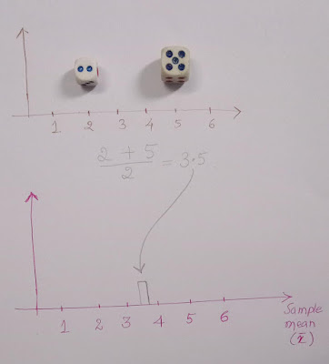
We got 2 and 5. The sample mean of 2 and 5 is 3.5.

 And the standard deviation of sample means is the population standard deviation divided by the square root of the sample size.

Let us plot the mean (3.5) as shown below in a plot.
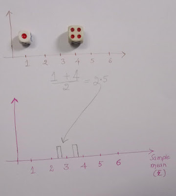
Round 2:
Now, we got 1 and 4. The mean of 1 and 4 is 2.5. Let us mark it in our plot.
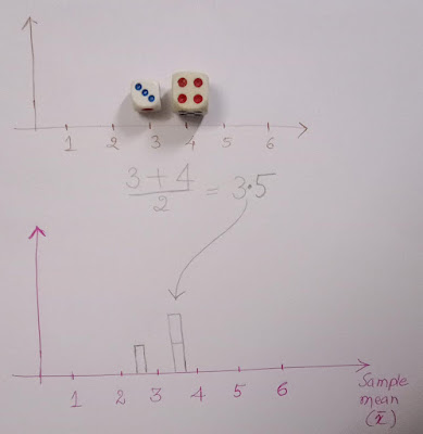
Round 3:
Then we got 3 and 4. The mean is 3.5. Let's mark the mean in our plot.
Round n:
Our plot where we marked all the sample means is called the sampling distribution of the mean. After many rounds, let us say 30 or 100 rounds, the sampling distribution of the mean approaches normal distribution.
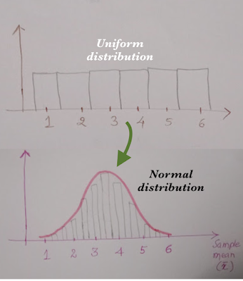
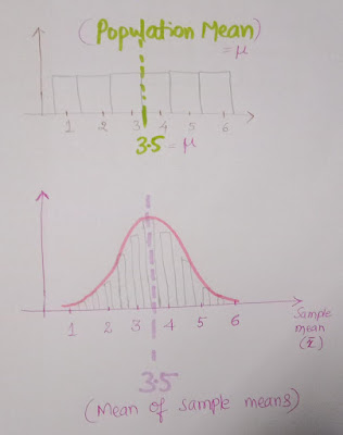
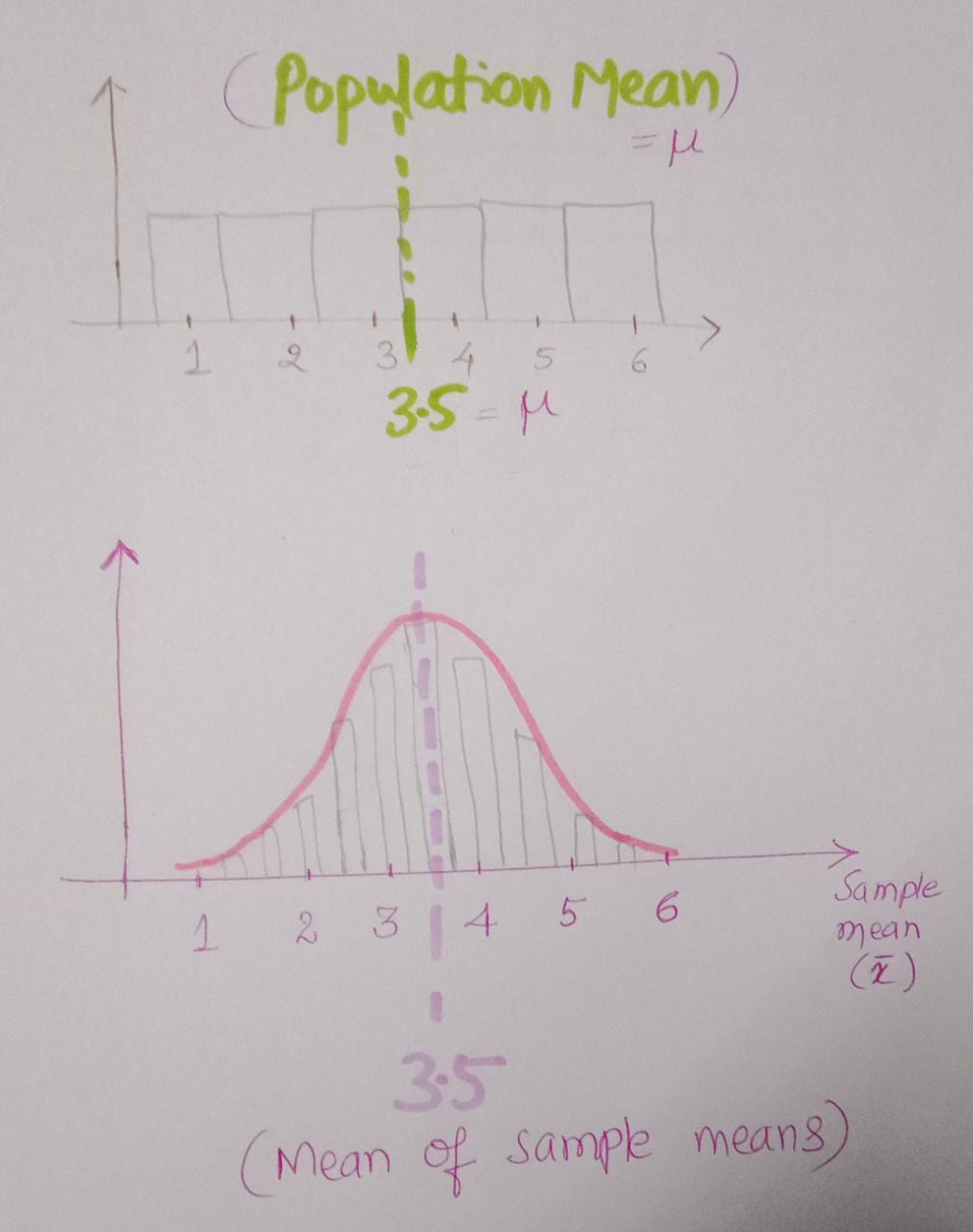
We know that by rolling a fair dice, all the values (1,2,3,4,5 & 6) have an equal chance: it follows a uniform distribution as shown below. Fair dice roll outcomes are independent and identically distributed (i.i.d.)
Even though the original data follows a uniform distribution, the sampling distribution of the mean follows a normal distribution.

In simple terms, Central Limit Theorem says that, regardless of the distribution of the data, sample means will be normally distributed for sufficiently large random samples.
Further, the mean of sample means = population mean, which is shown below.

In this blog post, we understood the concept of the Central Limit Theorem using examples.
No comments:
Post a Comment