Demystifying Degrees of Freedom with Visual Examples: A Beginner's Guide

The concept of degrees of freedom (df) is fundamental and commonly used in statistical analysis. In this blog post, let us thoroughly understand this concept with examples.

Many a time, you might have encountered that the degrees of freedom for a particular test is, let's say (n-1) or (n-2) etc. In the blog post, let us understand this concept with examples.

A) Without any restriction

Suppose I give you three boxes as shown below. You are free to fill all these three boxes with any values of your choice. Hence, in this case, the degrees of freedom are 3. In other words, df=n here.

B) With a restriction

Now let me modify the same example by imposing a restriction. The restriction is that you can fill these three boxes with any values but the summation should be 30.

Let us imagine you filled the first cell with 10. Now you are left with 2 boxes.

And you fill the second box with 5. Now as the sum should be 30, you have to fill the third cell with 15.

Hence, even though there were three cells, you were free to choose values for 2 cells. Hence, in this case, the degrees of freedom is 2. In other words, df=(n-1) here.

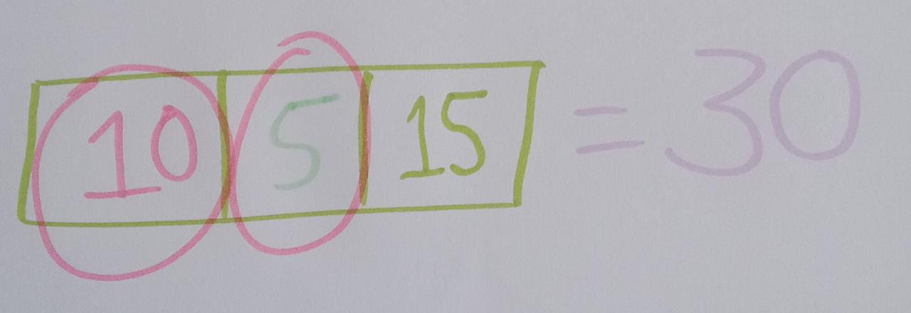
C) Degrees of freedom in contingency tables

In contingency tables, degrees of freedom are = (row-1)*(column-1). Let us understand this using different examples.

1) Degrees of freedom in 2x2 contingency table

Suppose you are given with a 2x2 table with row and column totals. You have to fill the values in four cells, but the row and column totals should be equal to the given values.

And you start with the first cell by filling it with 5. You now have no freedom to fill other values. Hence the degree of freedom is 1. Here, (row-1)*(column-1) = (2-1)*(2-1)= 1.

2) Degrees of freedom in 2x3 contingency table

Let us extend the same example to 2x3 table.

Imagine you filled the first cell with 5.

You are free to fill one more cell. And you fill it with 4. That's all. No more freedom. Hence, degrees of freedom is 2. Here, (row-1)*(column-1) = (2-1)*(3-1)= 2.

3) Degrees of freedom in 3x3 contingency table

Here, as you can see, you are free to fill 4 cells. Hence, degrees of freedom is 4. Here, (row-1)*(column-1) = (3-1)*(3-1)= 4.

D) Bessel's correction

The formula for estimating sample variance is given below. Sample variance is the square of the sample standard deviation.

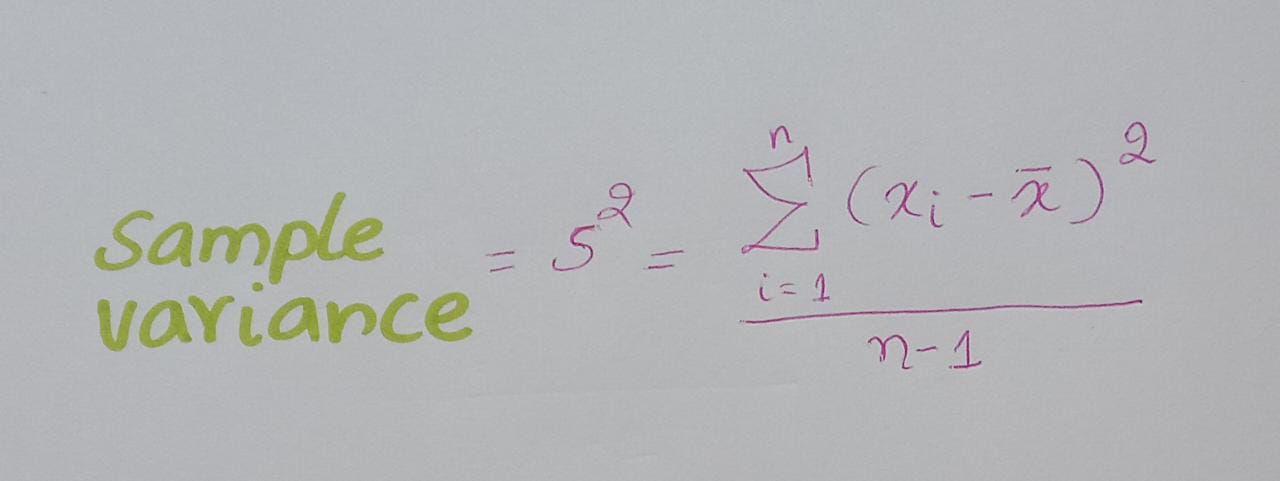
As you can see in the denominator, (n-1) is used instead of n.

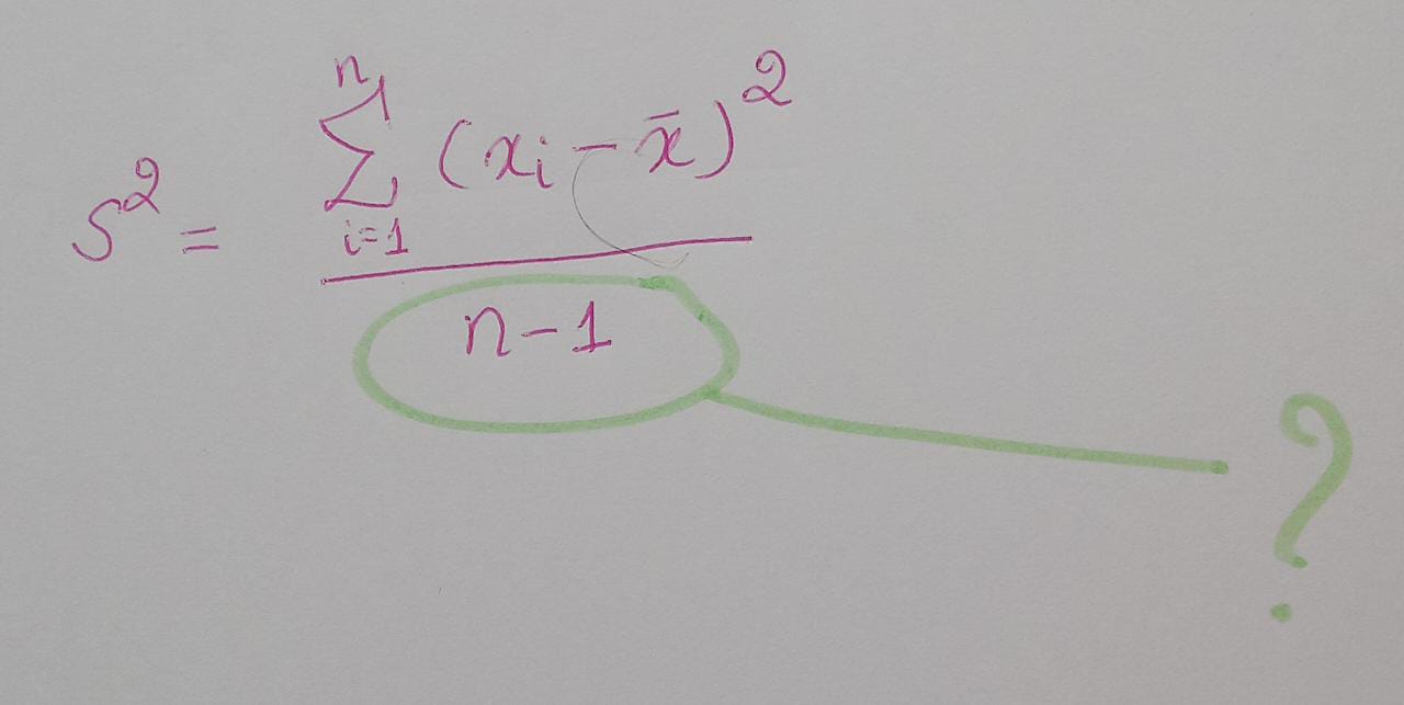
What could be the reason? When we are estimating sample variance (or the sample standard deviation), we also need sample mean. For estimating the sample mean, we have already used one of the degrees of freedom. 

Hence, now we are left with (n-1) degrees of freedom for estimating the sample variance (or the sample standard deviation). This is called Bessel's correction.

In summary, degrees of freedom = (sample size) - (number of parameters to be estimated).

You can watch the following video to know more: